An OLAP (OnLine Analytical Processing) cube is a multi‐dimensional database (ie. more than 2 dimensions) that allows fast analysis of data. OLTP databases, such as the Microsoft Dynamics AX 2009 database, are excellent for storing data, but not very efficient at analyzing large amounts of data. OLAP cubes are designed with analysis in mind, organizing data in a meaningful way, so that it can be accessed and analyzed quickly.
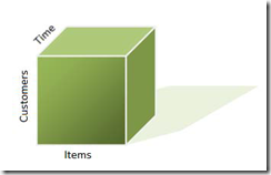
The term Cube comes from the most basic multi‐dimensional model of an OLAP database, ie. a three‐dimensional data structure. For example, Three dimensions of Items, Customers and Time:
This is a simple concept of OLAP data: being able to see items sold to customers on specific dates (or times). Such an OLAP cube would allow very fast analysis of this data, with intelligent filtering. For example: All items sold to a specific customer in last fiscal year; All customers who purchased a specific item in last quarter; Months where a particular item did not sell; Weeks where a particular customer did not purchase; Zip codes where a particular item sold the most in the period after a catalog delivery.
This is just an example cube structure with three dimensions. OLAP cubes can have more than three dimensions, exponentially expanding their data analysis potential. For example, we could add Employee to the previous cube example. Then we could find: Which employees sold a particular item during its promotional period, and to which customers?
When queried, SQL Server Analysis Services “slices and dices” the cubes, to find the data it needs. For example, it slices along the Customer dimension at the position of a particular customer, slices along the Item dimension at the position of a particular item, and it is left with a linear result along on the Time dimension (to see the purchasing history of a particular Customer for a particular Item).
Let’s introduce some common multi‐dimensional model terminology, with examples of their representation in BIDS:
• Dimension – this can be described as a category within the data, which would be reported on. For example: Time, Items, Customers, Employees, Sites, Warehouses, etc. In our BIDS project, there are 12 dimensions, and these can be seen in the Solution Explorer:
• Member – this is one point on a dimension. For example, Wednesday or October on the Time dimension, Customer ABC on the Customer dimension, John Citizen on the Employee dimension. This can be seen in BIDS, only after the cube has been processed (ie. contains data, and is not just a model).
• Calculated member – this is a member that is defined at run time.
• Attribute – this is a complete collection of Members. For example, all the days of the week, or all the months of the year, are attributes on the Time dimension. This can be seen in BIDS using the Dimension Designer. Here is are the attributes for the Time dimension:
• Attribute relationship – this is when one attribute relates to another. For example, the attribute Months on the Time dimension, is related to the attribute Quarters on the Time dimension.
• Tuple – this is a coordinate in the multi‐dimensional space. For example, in our previous three‐dimensional example, ([Item: ABC], [Customer: 111], [Time: October‐2008]) would be a tuple. Wild cards can also be used in tuples, and this is done by simply not including their values in the tuple. For example, ([ABC]) would represent sales of item ABC to all customers over all time. This would also represent a “slice” in the three‐dimensional model, along the ABC member on the Item dimension.
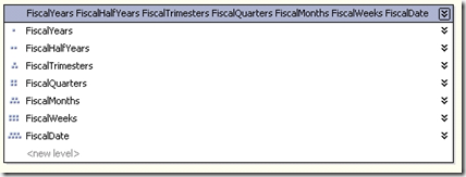
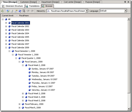
• Dimension hierarchies – these are used when a dimension has different groups of members that could be reported on. For example, on the Time dimension, some analysis may be done by year. Others may be done by Month, by Week, by Quarter, by Date, or by Day of the Week. To facilitate this, different dimension hierarchies can be defined. For example: Year, Quarter, Month, Week, Day; or, Year, Half‐Year, Trimester, Quarter, Month, Week, Date. This can be seen in the BIDS Dimension Designer only after the cube has been processed (since it relies on actual data values). Here are two examples of dimension hierarchies on the Time dimension. First, the hierarchy defined as “Years Quarters Months Weeks Days” (shown as design, then actual members):
Now the hierarchy defined as “FiscalYears FiscalHalfYears FiscalTrimesters FiscalQuarters FiscalMonths FiscalWeeks FiscalDate”:
Note that these hierarchies define different “scales” of members upon the same dimension. Another example would be a “Feet Inches” hierarchy and a “Meters Centimeters” hierarchy on the same Distance dimension.
• Measures – this describes the value, from a fact table, at a particular tuple. For example, at the tuple defined by ([ABC], [111], [October‐2008]) there could exist multiple values, such as quantity sold, amount paid, quantity returned, quantity delivered, etc. To define exactly which value is being analyzed, we use measures. Measures are stored in Measure groups. In BIDS, measures and measure groups can be seen in the Cube designer, like the Amount Settled measure, in the Customer Transactions measure group, shown below (with its property window):
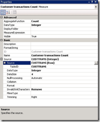
• Aggregation function – this is a function used on measures. For example, sum, count, average. In the previous example, you can see that the Amount Settled measure is using the Sum aggregate function, meaning its values will be summed when calculating total amounts. Here is another example. This time we look at the Customer transactions Count measure, which uses the Count aggregation function. So its values will be counted, not summed.


No comments:
Post a Comment